8. How-to discussions
This section describes how to perform common tasks using LIGGGHTS(R)-PUBLIC.
- Restarting a simulation
- 2d simulations
- Running multiple simulations from one input script
- Granular models
- Coupling LIGGGHTS(R)-PUBLIC to other codes
- Visualizing LIGGGHTS(R)-PUBLIC snapshots
- Triclinic (non-orthogonal) simulation boxes
- Output from LIGGGHTS(R)-PUBLIC (thermo, dumps, computes, fixes, variables)
- Walls
- Library interface to LIGGGHTS(R)-PUBLIC
The example input scripts included in the LIGGGHTS(R)-PUBLIC distribution and
highlighted in Section_example also show how to
setup and run various kinds of simulations.
8.1. Restarting a simulation
There are 3 ways to continue a long LIGGGHTS(R)-PUBLIC simulation. Multiple run commands can be used in the same input script. Each run will continue from where the previous run left off. Or binary restart files can be saved to disk using the restart command. At a later time, these binary files can be read via a read_restart command in a new script. Or they can be converted to text data files using the -r command-line switch and read by a read_data command in a new script.
The read_restart command typically replaces the “create_box”create_box.html command in the input script that restarts the simulation.
Note that while the internal state of the simulation is stored in the restart file, most material properties and simulation settings are not stored in the restart file. Be careful when changing settings and/or material parameters when restarting a simulation.
The following commands do not need to be repeated because their settings are included in the restart file: units, atom_style.
As an alternate approach, the restart file could be converted to a data file as follows:
lmp_g++ -r tmp.restart.50 tmp.restart.data
Then, the “read_data”read_data.html command can be used to restart the simulation.
reset_timestep command can be used to tell LIGGGHTS(R)-PUBLIC the current timestep.
8.2. 2d simulations
Use the dimension command to specify a 2d simulation.
Make the simulation box periodic in z via the boundary command. This is the default.
If using the create box command to define a simulation box, set the z dimensions narrow, but finite, so that the create_atoms command will tile the 3d simulation box with a single z plane of atoms - e.g.
create box 1 -10 10 -10 10 -0.25 0.25
If using the read data command to read in a file of atom coordinates, set the “zlo zhi” values to be finite but narrow, similar to the create_box command settings just described. For each atom in the file, assign a z coordinate so it falls inside the z-boundaries of the box - e.g. 0.0.
Use the fix enforce2d command as the last defined fix to insure that the z-components of velocities and forces are zeroed out every timestep. The reason to make it the last fix is so that any forces induced by other fixes will be zeroed out.
Many of the example input scripts included in the LIGGGHTS(R)-PUBLIC distribution are for 2d models.
Warning
Some models in LIGGGHTS(R)-PUBLIC treat particles as finite-size spheres, as opposed to point particles. In 2d, the particles will still be spheres, not disks, meaning their moment of inertia will be the same as in 3d.
8.3. Running multiple simulations from one input script
This can be done in several ways. See the documentation for individual commands for more details on how these examples work.
If “multiple simulations” means continue a previous simulation for more timesteps, then you simply use the run command multiple times. For example, this script
units lj
atom_style atomic
read_data data.lj
run 10000
run 10000
run 10000
run 10000
run 10000
would run 5 successive simulations of the same system for a total of 50,000 timesteps.
If you wish to run totally different simulations, one after the other, the clear command can be used in between them to re-initialize LIGGGHTS(R)-PUBLIC. For example, this script
units lj
atom_style atomic
read_data data.lj
run 10000
clear
units lj
atom_style atomic
read_data data.lj.new
run 10000
would run 2 independent simulations, one after the other.
For large numbers of independent simulations, you can use variables and the next and jump commands to loop over the same input script multiple times with different settings. For example, this script, named in.polymer
variable d index run1 run2 run3 run4 run5 run6 run7 run8
shell cd $d
read_data data.polymer
run 10000
shell cd ..
clear
next d
jump in.polymer
would run 8 simulations in different directories, using a data.polymer file in each directory. The same concept could be used to run the same system at 8 different temperatures, using a temperature variable and storing the output in different log and dump files, for example
variable a loop 8
variable t index 0.8 0.85 0.9 0.95 1.0 1.05 1.1 1.15
log log.$a
read data.polymer
velocity all create $t 352839
fix 1 all nvt $t $t 100.0
dump 1 all atom 1000 dump.$a
run 100000
next t
next a
jump in.polymer
All of the above examples work whether you are running on 1 or multiple processors, but assumed you are running LIGGGHTS(R)-PUBLIC on a single partition of processors. LIGGGHTS(R)-PUBLIC can be run on multiple partitions via the “-partition” command-line switch as described in this section of the manual.
In the last 2 examples, if LIGGGHTS(R)-PUBLIC were run on 3 partitions, the same scripts could be used if the “index” and “loop” variables were replaced with universe-style variables, as described in the variable command. Also, the “next t” and “next a” commands would need to be replaced with a single “next a t” command. With these modifications, the 8 simulations of each script would run on the 3 partitions one after the other until all were finished. Initially, 3 simulations would be started simultaneously, one on each partition. When one finished, that partition would then start the 4th simulation, and so forth, until all 8 were completed.
8.4. Granular models
Granular system are composed of spherical particles with a diameter, as opposed to point particles. This means they have an angular velocity and torque can be imparted to them to cause them to rotate.
To run a simulation of a granular model, you will want to use the following commands:
This compute
calculates rotational kinetic energy which can be output with thermodynamic info.
Use a number of particle-particle and particle-wall contact models, which compute forces and torques between interacting pairs of particles and between particles and primitive walls or mesh elements. Details can be found here:
These commands implement fix options specific to granular systems:
- fix freeze
fix pour- fix viscous
- fix wall/gran
fix wall/gran commands can define two types of walls: primitive and mesh. Mesh walls are defined using a fix mesh/surface or related command.
The fix style freeze zeroes both the force and torque of frozen atoms, and should be used for granular system instead of the fix style setforce.
For computational efficiency, you can eliminate needless pairwise computations between frozen atoms by using this command:
- neigh_modify exclude
8.5. Coupling LIGGGHTS(R)-PUBLIC to other codes
LIGGGHTS(R)-PUBLIC is designed to allow it to be coupled to other codes. For example, a quantum mechanics code might compute forces on a subset of atoms and pass those forces to LIGGGHTS(R)-PUBLIC. Or a continuum finite element (FE) simulation might use atom positions as boundary conditions on FE nodal points, compute a FE solution, and return interpolated forces on MD atoms.
LIGGGHTS(R)-PUBLIC can be coupled to other codes in at least 3 ways. Each has advantages and disadvantages, which you’ll have to think about in the context of your application.
(1) Define a new fix command that calls the other code. In this scenario, LIGGGHTS(R)-PUBLIC is the driver code. During its timestepping, the fix is invoked, and can make library calls to the other code, which has been linked to LIGGGHTS(R)-PUBLIC as a library. This is the way the POEMS package that performs constrained rigid-body motion on groups of atoms is hooked to LIGGGHTS(R)-PUBLIC. See the fix_poems command for more details. See this section of the documentation for info on how to add a new fix to LIGGGHTS(R)-PUBLIC.
(2) Define a new LIGGGHTS(R)-PUBLIC command that calls the other code. This is conceptually similar to method (1), but in this case LIGGGHTS(R)-PUBLIC and the other code are on a more equal footing. Note that now the other code is not called during the timestepping of a LIGGGHTS(R)-PUBLIC run, but between runs. The LIGGGHTS(R)-PUBLIC input script can be used to alternate LIGGGHTS(R)-PUBLIC runs with calls to the other code, invoked via the new command. The run command facilitates this with its every option, which makes it easy to run a few steps, invoke the command, run a few steps, invoke the command, etc.
In this scenario, the other code can be called as a library, as in (1), or it could be a stand-alone code, invoked by a system() call made by the command (assuming your parallel machine allows one or more processors to start up another program). In the latter case the stand-alone code could communicate with LIGGGHTS(R)-PUBLIC thru files that the command writes and reads.
See Section_modify of the documentation for how to add a new command to LIGGGHTS(R)-PUBLIC.
(3) Use LIGGGHTS(R)-PUBLIC as a library called by another code. In this case the other code is the driver and calls LIGGGHTS(R)-PUBLIC as needed. Or a wrapper code could link and call both LIGGGHTS(R)-PUBLIC and another code as libraries. Again, the run command has options that allow it to be invoked with minimal overhead (no setup or clean-up) if you wish to do multiple short runs, driven by another program.
Examples of driver codes that call LIGGGHTS(R)-PUBLIC as a library are included in the examples/COUPLE directory of the LIGGGHTS(R)-PUBLIC distribution; see examples/COUPLE/README for more details:
- simple: simple driver programs in C++ and C which invoke LIGGGHTS(R)-PUBLIC as a library
- lammps_quest: coupling of LIGGGHTS(R)-PUBLIC and Quest, to run classical MD with quantum forces calculated by a density functional code
- lammps_spparks: coupling of LIGGGHTS(R)-PUBLIC and SPPARKS, to couple a kinetic Monte Carlo model for grain growth using MD to calculate strain induced across grain boundaries
This section of the documentation describes how to build LIGGGHTS(R)-PUBLIC as a library. Once this is done, you can interface with LIGGGHTS(R)-PUBLIC either via C++, C, Fortran, or Python (or any other language that supports a vanilla C-like interface). For example, from C++ you could create one (or more) “instances” of LIGGGHTS(R)-PUBLIC, pass it an input script to process, or execute individual commands, all by invoking the correct class methods in LIGGGHTS(R)-PUBLIC. From C or Fortran you can make function calls to do the same things. See Section_python of the manual for a description of the Python wrapper provided with LIGGGHTS(R)-PUBLIC that operates through the LIGGGHTS(R)-PUBLIC library interface.
The files src/library.cpp and library.h contain the C-style interface to LIGGGHTS(R)-PUBLIC. See Section_howto 19 of the manual for a description of the interface and how to extend it for your needs.
Note that the lammps_open() function that creates an instance of LIGGGHTS(R)-PUBLIC takes an MPI communicator as an argument. This means that instance of LIGGGHTS(R)-PUBLIC will run on the set of processors in the communicator. Thus the calling code can run LIGGGHTS(R)-PUBLIC on all or a subset of processors. For example, a wrapper script might decide to alternate between LIGGGHTS(R)-PUBLIC and another code, allowing them both to run on all the processors. Or it might allocate half the processors to LIGGGHTS(R)-PUBLIC and half to the other code and run both codes simultaneously before syncing them up periodically. Or it might instantiate multiple instances of LIGGGHTS(R)-PUBLIC to perform different calculations.
8.6. Visualizing LIGGGHTS(R)-PUBLIC snapshots
LIGGGHTS(R)-PUBLIC itself does not do visualization, but snapshots from LIGGGHTS(R)-PUBLIC simulations can be visualized (and analyzed) in a variety of ways.
LIGGGHTS(R)-PUBLIC snapshots are created by the dump command which can create files in several formats. The native LIGGGHTS(R)-PUBLIC dump format is a text file (see “dump atom” or “dump custom”).
A Python-based toolkit (LPP) distributed by our group can read native LIGGGHTS(R)-PUBLIC dump files, including custom dump files with additional columns of user-specified atom information, and convert them to VTK file formats that can be read with Paraview.
Also, there exist a number of dump commands that output to VTK natively.
8.7. Triclinic (non-orthogonal) simulation boxes
By default, LIGGGHTS(R)-PUBLIC uses an orthogonal simulation box to encompass the particles. The boundary command sets the boundary conditions of the box (periodic, non-periodic, etc). The orthogonal box has its “origin” at (xlo,ylo,zlo) and is defined by 3 edge vectors starting from the origin given by a = (xhi-xlo,0,0); b = (0,yhi-ylo,0); c = (0,0,zhi-zlo). The 6 parameters (xlo,xhi,ylo,yhi,zlo,zhi) are defined at the time the simulation box is created, e.g. by the create_box or read_data or read_restart commands. Additionally, LIGGGHTS(R)-PUBLIC defines box size parameters lx,ly,lz where lx = xhi-xlo, and similarly in the y and z dimensions. The 6 parameters, as well as lx,ly,lz, can be output via the thermo_style custom command.
LIGGGHTS(R)-PUBLIC also allows simulations to be performed in triclinic (non-orthogonal) simulation boxes shaped as a parallelepiped with triclinic symmetry. The parallelepiped has its “origin” at (xlo,ylo,zlo) and is defined by 3 edge vectors starting from the origin given by a = (xhi-xlo,0,0); b = (xy,yhi-ylo,0); c = (xz,yz,zhi-zlo). xy,xz,yz can be 0.0 or positive or negative values and are called “tilt factors” because they are the amount of displacement applied to faces of an originally orthogonal box to transform it into the parallelepiped. In LIGGGHTS(R)-PUBLIC the triclinic simulation box edge vectors a, b, and c cannot be arbitrary vectors. As indicated, a must lie on the positive x axis. b must lie in the xy plane, with strictly positive y component. c may have any orientation with strictly positive z component. The requirement that a, b, and c have strictly positive x, y, and z components, respectively, ensures that a, b, and c form a complete right-handed basis. These restrictions impose no loss of generality, since it is possible to rotate/invert any set of 3 crystal basis vectors so that they conform to the restrictions.
For example, assume that the 3 vectors A,**B**,**C** are the edge vectors of a general parallelepiped, where there is no restriction on A,**B**,**C** other than they form a complete right-handed basis i.e. A x B . C > 0. The equivalent LIGGGHTS(R)-PUBLIC a,**b**,**c** are a linear rotation of A, B, and C and can be computed as follows:
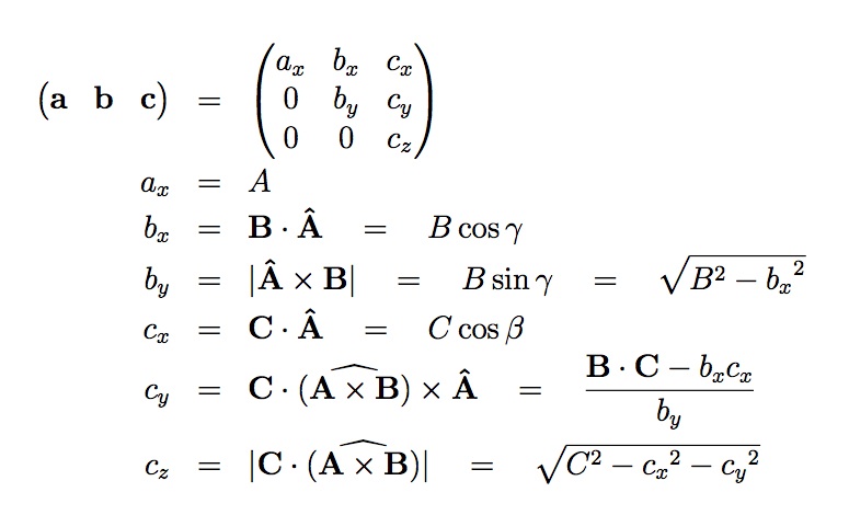
where A = |**A**| indicates the scalar length of A. The ^ hat symbol indicates the corresponding unit vector. beta and gamma are angles between the vectors described below. Note that by construction, a, b, and c have strictly positive x, y, and z components, respectively. If it should happen that A, B, and C form a left-handed basis, then the above equations are not valid for c. In this case, it is necessary to first apply an inversion. This can be achieved by interchanging two basis vectors or by changing the sign of one of them.
For consistency, the same rotation/inversion applied to the basis vectors must also be applied to atom positions, velocities, and any other vector quantities. This can be conveniently achieved by first converting to fractional coordinates in the old basis and then converting to distance coordinates in the new basis. The transformation is given by the following equation:
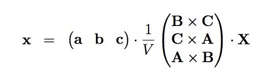
where V is the volume of the box, X is the original vector quantity and x is the vector in the LIGGGHTS(R)-PUBLIC basis.
There is no requirement that a triclinic box be periodic in any
dimension, though it typically should be in at least the 2nd dimension
of the tilt (y in xy) if you want to enforce a shift in periodic
boundary conditions across that boundary. Some commands that work
with triclinic boxes, e.g. the fix deform and fix npt commands, require periodicity or non-shrink-wrap
boundary conditions in specific dimensions. See the command doc pages
for details.
The 9 parameters (xlo,xhi,ylo,yhi,zlo,zhi,xy,xz,yz) are defined at the time the simluation box is created. This happens in one of 3 ways. If the create_box command is used with a region of style prism, then a triclinic box is setup. See the region command for details. If the read_data command is used to define the simulation box, and the header of the data file contains a line with the “xy xz yz” keyword, then a triclinic box is setup. See the read_data command for details. Finally, if the read_restart command reads a restart file which was written from a simulation using a triclinic box, then a triclinic box will be setup for the restarted simulation.
Note that you can define a triclinic box with all 3 tilt factors =
0.0, so that it is initially orthogonal. This is necessary if the box
will become non-orthogonal, e.g. due to the fix npt or
fix deform commands. Alternatively, you can use the
change_box command to convert a simulation box from
orthogonal to triclinic and vice versa.
As with orthogonal boxes, LIGGGHTS(R)-PUBLIC defines triclinic box size parameters lx,ly,lz where lx = xhi-xlo, and similarly in the y and z dimensions. The 9 parameters, as well as lx,ly,lz, can be output via the thermo_style custom command.
To avoid extremely tilted boxes (which would be computationally inefficient), LIGGGHTS(R)-PUBLIC normally requires that no tilt factor can skew the box more than half the distance of the parallel box length, which is the 1st dimension in the tilt factor (x for xz). This is required both when the simulation box is created, e.g. via the create_box or read_data commands, as well as when the box shape changes dynamically during a simulation, e.g. via the fix deform command.
For example, if xlo = 2 and xhi = 12, then the x box length is 10 and the xy tilt factor must be between -5 and 5. Similarly, both xz and yz must be between -(xhi-xlo)/2 and +(yhi-ylo)/2. Note that this is not a limitation, since if the maximum tilt factor is 5 (as in this example), then configurations with tilt = ..., -15, -5, 5, 15, 25, ... are geometrically all equivalent. If the box tilt exceeds this limit during a dynamics run (e.g. via the fix deform command), then the box is “flipped” to an equivalent shape with a tilt factor within the bounds, so the run can continue. See the fix deform doc page for further details.
One exception to this rule is if the 1st dimension in the tilt factor (x for xy) is non-periodic. In that case, the limits on the tilt factor are not enforced, since flipping the box in that dimension does not change the atom positions due to non-periodicity. In this mode, if you tilt the system to extreme angles, the simulation will simply become inefficient, due to the highly skewed simulation box.
The limitation on not creating a simulation box with a tilt factor skewing the box more than half the distance of the parallel box length can be overridden via the box command. Setting the tilt keyword to large allows any tilt factors to be specified.
Note that if a simulation box has a large tilt factor, LIGGGHTS(R)-PUBLIC will run less efficiently, due to the large volume of communication needed to acquire ghost atoms around a processor’s irregular-shaped sub-domain. For extreme values of tilt, LIGGGHTS(R)-PUBLIC may also lose atoms and generate an error.
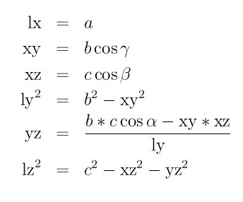
Triclinic crystal structures are often defined using three lattice constants a, b, and c, and three angles alpha, beta and gamma. Note that in this nomenclature, the a, b, and c lattice constants are the scalar lengths of the edge vectors a, b, and c defined above. The relationship between these 6 quantities (a,b,c,alpha,beta,gamma) and the LIGGGHTS(R)-PUBLIC box sizes (lx,ly,lz) = (xhi-xlo,yhi-ylo,zhi-zlo) and tilt factors (xy,xz,yz) is as follows:
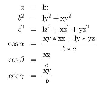
The inverse relationship can be written as follows:
The values of a, b, c , alpha, beta , and gamma can be printed out or accessed by computes using the thermo_style custom keywords cella, cellb, cellc, cellalpha, cellbeta, cellgamma, respectively.
As discussed on the dump command doc page, when the BOX BOUNDS for a snapshot is written to a dump file for a triclinic box, an orthogonal bounding box which encloses the triclinic simulation box is output, along with the 3 tilt factors (xy, xz, yz) of the triclinic box, formatted as follows:
ITEM: BOX BOUNDS xy xz yz
xlo_bound xhi_bound xy
ylo_bound yhi_bound xz
zlo_bound zhi_bound yz
This bounding box is convenient for many visualization programs and is calculated from the 9 triclinic box parameters (xlo,xhi,ylo,yhi,zlo,zhi,xy,xz,yz) as follows:
xlo_bound = xlo + MIN(0.0,xy,xz,xy+xz)
xhi_bound = xhi + MAX(0.0,xy,xz,xy+xz)
ylo_bound = ylo + MIN(0.0,yz)
yhi_bound = yhi + MAX(0.0,yz)
zlo_bound = zlo
zhi_bound = zhi
These formulas can be inverted if you need to convert the bounding box back into the triclinic box parameters, e.g. xlo = xlo_bound - MIN(0.0,xy,xz,xy+xz).
8.8. Output from LIGGGHTS(R)-PUBLIC (thermo, dumps, computes, fixes, variables)
There are four basic kinds of LIGGGHTS(R)-PUBLIC output:
- Thermodynamic output, which is a list of quantities printed every few timesteps to the screen and logfile.
- Dump files, which contain snapshots of atoms and various per-atom values and are written at a specified frequency.
- Certain fixes can output user-specified quantities to files: fix ave/time for time averaging, fix ave/spatial for spatial averaging, and fix print for single-line output of variables. Fix print can also output to the screen.
- Restart files.
A simulation prints one set of thermodynamic output and (optionally) restart files. It can generate any number of dump files and fix output files, depending on what dump and fix commands you specify.
As discussed below, LIGGGHTS(R)-PUBLIC gives you a variety of ways to determine what quantities are computed and printed when the thermodynamics, dump, or fix commands listed above perform output. Throughout this discussion, note that users can also add their own computes and fixes to LIGGGHTS(R)-PUBLIC which can then generate values that can then be output with these commands.
The following sub-sections discuss different LIGGGHTS(R)-PUBLIC command related to output and the kind of data they operate on and produce:
- Global/per-atom/local data
- Scalar/vector/array data
- Thermodynamic output
- Dump file output
- Fixes that write output files
- Computes that process output quantities
- Fixes that process output quantities
- Computes that generate values to output
- Fixes that generate values to output
- Variables that generate values to output
- Summary table of output options and data flow between commands
8.8.1. Global/per-atom/local data
Various output-related commands work with three different styles of data: global, per-atom, or local. A global datum is one or more system-wide values, e.g. the temperature of the system. A per-atom datum is one or more values per atom, e.g. the kinetic energy of each atom. Local datums are calculated by each processor based on the atoms it owns, but there may be zero or more per atom, e.g. a list of bond distances.
8.8.2. Scalar/vector/array data
Global, per-atom, and local datums can each come in three kinds: a single scalar value, a vector of values, or a 2d array of values. The doc page for a “compute” or “fix” or “variable” that generates data will specify both the style and kind of data it produces, e.g. a per-atom vector.
When a quantity is accessed, as in many of the output commands discussed below, it can be referenced via the following bracket notation, where ID in this case is the ID of a compute. The leading “c_” would be replaced by “f_” for a fix, or “v_” for a variable:
| c_ID | entire scalar, vector, or array |
| c_ID[I] | one element of vector, one column of array |
| c_ID[I][J] | one element of array |
In other words, using one bracket reduces the dimension of the data once (vector -> scalar, array -> vector). Using two brackets reduces the dimension twice (array -> scalar). Thus a command that uses scalar values as input can typically also process elements of a vector or array.
8.8.3. Thermodynamic output
The frequency and format of thermodynamic output is set by the thermo, thermo_style, and thermo_modify commands. The thermo_style command also specifies what values are calculated and written out. Pre-defined keywords can be specified (e.g. press, etotal, etc). Three additional kinds of keywords can also be specified (c_ID, f_ID, v_name), where a compute or fix or variable provides the value to be output. In each case, the compute, fix, or variable must generate global values for input to the thermo_style custom command.
Note that thermodynamic output values can be “extensive” or “intensive”. The former scale with the number of atoms in the system (e.g. total energy), the latter do not (e.g. temperature). The setting for thermo_modify norm determines whether extensive quantities are normalized or not. Computes and fixes produce either extensive or intensive values; see their individual doc pages for details. Equal-style variables produce only intensive values; you can include a division by “natoms” in the formula if desired, to make an extensive calculation produce an intensive result.
8.8.4. Dump file output
Dump file output is specified by the dump and dump_modify commands. There are several pre-defined formats (dump atom, dump xtc, etc).
There is also a dump custom format where the user specifies what values are output with each atom. Pre-defined atom attributes can be specified (id, x, fx, etc). Three additional kinds of keywords can also be specified (c_ID, f_ID, v_name), where a compute or fix or variable provides the values to be output. In each case, the compute, fix, or variable must generate per-atom values for input to the dump custom command.
There is also a dump local format where the user specifies what local values to output. A pre-defined index keyword can be specified to enumuerate the local values. Two additional kinds of keywords can also be specified (c_ID, f_ID), where a compute or fix or variable provides the values to be output. In each case, the compute or fix must generate local values for input to the dump local command.
8.8.5. Fixes that write output files
Several fixes take various quantities as input and can write output files: fix ave/time, fix ave/spatial, fix ave/histo, fix ave/correlate, and fix print.
The fix ave/time command enables direct output to a file and/or time-averaging of global scalars or vectors. The user specifies one or more quantities as input. These can be global compute values, global fix values, or variables of any style except the atom style which produces per-atom values. Since a variable can refer to keywords used by the thermo_style custom command (like temp or press) and individual per-atom values, a wide variety of quantities can be time averaged and/or output in this way. If the inputs are one or more scalar values, then the fix generate a global scalar or vector of output. If the inputs are one or more vector values, then the fix generates a global vector or array of output. The time-averaged output of this fix can also be used as input to other output commands.
The fix ave/spatial command enables direct output to a file of spatial-averaged per-atom quantities like those output in dump files, within 1d layers of the simulation box. The per-atom quantities can be atom density (mass or number) or atom attributes such as position, velocity, force. They can also be per-atom quantities calculated by a compute, by a fix, or by an atom-style variable. The spatial-averaged output of this fix can also be used as input to other output commands.
The fix ave/histo command enables direct output to a file of histogrammed quantities, which can be global or per-atom or local quantities. The histogram output of this fix can also be used as input to other output commands.
The fix ave/correlate command enables direct output to a file of time-correlated quantities, which can be global scalars. The correlation matrix output of this fix can also be used as input to other output commands.
The fix print command can generate a line of output written to the screen and log file or to a separate file, periodically during a running simulation. The line can contain one or more variable values for any style variable except the atom style). As explained above, variables themselves can contain references to global values generated by thermodynamic keywords, computes, fixes, or other variables, or to per-atom values for a specific atom. Thus the fix print command is a means to output a wide variety of quantities separate from normal thermodynamic or dump file output.
8.8.6. Computes that process output quantities
The compute reduce and compute reduce/region commands take one or more per-atom or local vector quantities as inputs and “reduce” them (sum, min, max, ave) to scalar quantities. These are produced as output values which can be used as input to other output commands.
The compute slice command take one or more global vector or array quantities as inputs and extracts a subset of their values to create a new vector or array. These are produced as output values which can be used as input to other output commands.
The compute property/atom command takes a list of one or more pre-defined atom attributes (id, x, fx, etc) and stores the values in a per-atom vector or array. These are produced as output values which can be used as input to other output commands. The list of atom attributes is the same as for the dump custom command.
The compute property/local command takes a list of one or more pre-defined local attributes (bond info, angle info, etc) and stores the values in a local vector or array. These are produced as output values which can be used as input to other output commands.
The compute atom/molecule command takes a list of one or more per-atom quantities (from a compute, fix, per-atom variable) and sums the quantities on a per-molecule basis. It produces a global vector or array as output values which can be used as input to other output commands.
8.8.7. Fixes that process output quantities
The fix ave/atom command performs time-averaging of per-atom vectors. The per-atom quantities can be atom attributes such as position, velocity, force. They can also be per-atom quantities calculated by a compute, by a fix, or by an atom-style variable. The time-averaged per-atom output of this fix can be used as input to other output commands.
The fix store/state command can archive one or more per-atom attributes at a particular time, so that the old values can be used in a future calculation or output. The list of atom attributes is the same as for the dump custom command, including per-atom quantities calculated by a compute, by a fix, or by an atom-style variable. The output of this fix can be used as input to other output commands.
8.8.8. Computes that generate values to output
Every compute in LIGGGHTS(R)-PUBLIC produces either global or per-atom or local values. The values can be scalars or vectors or arrays of data. These values can be output using the other commands described in this section. The doc page for each compute command describes what it produces. Computes that produce per-atom or local values have the word “atom” or “local” in their style name. Computes without the word “atom” or “local” produce global values.
8.8.9. Fixes that generate values to output
Some fixes in LIGGGHTS(R)-PUBLIC produces either global or per-atom or local values which can be accessed by other commands. The values can be scalars or vectors or arrays of data. These values can be output using the other commands described in this section. The doc page for each fix command tells whether it produces any output quantities and describes them.
8.8.10. Variables that generate values to output
Every variables defined in an input script generates either a global scalar value or a per-atom vector (only atom-style variables) when it is accessed. The formulas used to define equal- and atom-style variables can contain references to the thermodynamic keywords and to global and per-atom data generated by computes, fixes, and other variables. The values generated by variables can be output using the other commands described in this section.
8.8.11. Summary table of output options and data flow between commands
This table summarizes the various commands that can be used for generating output from LIGGGHTS(R)-PUBLIC. Each command produces output data of some kind and/or writes data to a file. Most of the commands can take data from other commands as input. Thus you can link many of these commands together in pipeline form, where data produced by one command is used as input to another command and eventually written to the screen or to a file. Note that to hook two commands together the output and input data types must match, e.g. global/per-atom/local data and scalar/vector/array data.
Also note that, as described above, when a command takes a scalar as input, that could be an element of a vector or array. Likewise a vector input could be a column of an array.
| Command | Input | Output | |
| thermo_style custom | global scalars | screen, log file | |
| dump custom | per-atom vectors | dump file | |
| dump local | local vectors | dump file | |
| fix print | global scalar from variable | screen, file | |
| global scalar from variable | screen | ||
| computes | N/A | global/per-atom/local scalar/vector/array | |
| fixes | N/A | global/per-atom/local scalar/vector/array | |
| variables | global scalars, per-atom vectors | global scalar, per-atom vector | |
| compute reduce | per-atom/local vectors | global scalar/vector | |
| compute slice | global vectors/arrays | global vector/array | |
| compute property/atom | per-atom vectors | per-atom vector/array | |
| compute property/local | local vectors | local vector/array | |
| compute atom/molecule | per-atom vectors | global vector/array | |
| fix ave/atom | per-atom vectors | per-atom vector/array | |
| fix ave/time | global scalars/vectors | global scalar/vector/array, file | |
| fix ave/spatial | per-atom vectors | global array, file | |
| fix ave/histo | global/per-atom/local scalars and vectors | global array, file | |
| fix ave/correlate | global scalars | global array, file | |
| fix store/state | per-atom vectors | per-atom vector/array | |
8.9. Walls
Walls are typically used to bound particle motion, i.e. to serve as a boundary condition.
Walls in LIGGGHTS(R)-PUBLIC for granular simulations are typically defined using fix wall/gran. This command can define two types of walls: primitive and mesh. Mesh walls are defined using a fix mesh/surface or related command.
Also. walls can be constructed made of particles
Rough walls, built of particles, can be created in various ways. The particles themselves can be generated like any other particle, via the lattice and create_atoms commands, or read in via the read_data command.
Their motion can be constrained by many different commands, so that they do not move at all, move together as a group at constant velocity or in response to a net force acting on them, move in a prescribed fashion (e.g. rotate around a point), etc. Note that if a time integration fix like fix nve is not used with the group that contains wall particles, their positions and velocities will not be updated.
- fix aveforce - set force on particles to average value, so they move together
- fix setforce - set force on particles to a value, e.g. 0.0
- fix freeze - freeze particles for use as granular walls
- fix nve/noforce - advect particles by their velocity, but without force
- fix move - prescribe motion of particles by a linear velocity, oscillation, rotation, variable
The fix move command offers the most generality, since the motion of individual particles can be specified with variable formula which depends on time and/or the particle position.
For rough walls, it may be useful to turn off pairwise interactions between wall particles via the neigh_modify exclude command.
Rough walls can also be created by specifying frozen particles that do not move and do not interact with mobile particles, and then tethering other particles to the fixed particles, via a bond. The bonded particles do interact with other mobile particles.
- fix wall/reflect - reflective flat walls
- fix wall/region - use region surface as wall
The fix wall/region command offers the most generality, since the region surface is treated as a wall, and the geometry of the region can be a simple primitive volume (e.g. a sphere, or cube, or plane), or a complex volume made from the union and intersection of primitive volumes. Regions can also specify a volume “interior” or “exterior” to the specified primitive shape or union or intersection. Regions can also be “dynamic” meaning they move with constant velocity, oscillate, or rotate.
8.10. Library interface to LIGGGHTS(R)-PUBLIC
As described in Section_start 5, LIGGGHTS(R)-PUBLIC can be built as a library, so that it can be called by another code, used in a coupled manner with other codes, or driven through a Python interface.
All of these methodologies use a C-style interface to LIGGGHTS(R)-PUBLIC that is provided in the files src/library.cpp and src/library.h. The functions therein have a C-style argument list, but contain C++ code you could write yourself in a C++ application that was invoking LIGGGHTS(R)-PUBLIC directly. The C++ code in the functions illustrates how to invoke internal LIGGGHTS(R)-PUBLIC operations. Note that LIGGGHTS(R)-PUBLIC classes are defined within a LIGGGHTS(R)-PUBLIC namespace (LAMMPS_NS) if you use them from another C++ application.
Library.cpp contains these 4 functions:
void lammps_open(int, char **, MPI_Comm, void **);
void lammps_close(void *);
void lammps_file(void *, char *);
char *lammps_command(void *, char *);
The lammps_open() function is used to initialize LIGGGHTS(R)-PUBLIC, passing in a list of strings as if they were command-line arguments when LIGGGHTS(R)-PUBLIC is run in stand-alone mode from the command line, and a MPI communicator for LIGGGHTS(R)-PUBLIC to run under. It returns a ptr to the LIGGGHTS(R)-PUBLIC object that is created, and which is used in subsequent library calls. The lammps_open() function can be called multiple times, to create multiple instances of LIGGGHTS(R)-PUBLIC.
LIGGGHTS(R)-PUBLIC will run on the set of processors in the communicator. This means the calling code can run LIGGGHTS(R)-PUBLIC on all or a subset of processors. For example, a wrapper script might decide to alternate between LIGGGHTS(R)-PUBLIC and another code, allowing them both to run on all the processors. Or it might allocate half the processors to LIGGGHTS(R)-PUBLIC and half to the other code and run both codes simultaneously before syncing them up periodically. Or it might instantiate multiple instances of LIGGGHTS(R)-PUBLIC to perform different calculations.
The lammps_close() function is used to shut down an instance of LIGGGHTS(R)-PUBLIC and free all its memory.
The lammps_file() and lammps_command() functions are used to pass a file or string to LIGGGHTS(R)-PUBLIC as if it were an input script or single command in an input script. Thus the calling code can read or generate a series of LIGGGHTS(R)-PUBLIC commands one line at a time and pass it thru the library interface to setup a problem and then run it, interleaving the lammps_command() calls with other calls to extract information from LIGGGHTS(R)-PUBLIC, perform its own operations, or call another code’s library.
Other useful functions are also included in library.cpp. For example:
void *lammps_extract_global(void *, char *)
void *lammps_extract_atom(void *, char *)
void *lammps_extract_compute(void *, char *, int, int)
void *lammps_extract_fix(void *, char *, int, int, int, int)
void *lammps_extract_variable(void *, char *, char *)
int lammps_get_natoms(void *)
void lammps_get_coords(void *, double *)
void lammps_put_coords(void *, double *)
These can extract various global or per-atom quantities from LIGGGHTS(R)-PUBLIC as well as values calculated by a compute, fix, or variable. The “get” and “put” operations can retrieve and reset atom coordinates. See the library.cpp file and its associated header file library.h for details.
The key idea of the library interface is that you can write any functions you wish to define how your code talks to LIGGGHTS(R)-PUBLIC and add them to src/library.cpp and src/library.h, as well as to the Python interface. The routines you add can access or change any LIGGGHTS(R)-PUBLIC data you wish. The examples/COUPLE and python directories have example C++ and C and Python codes which show how a driver code can link to LIGGGHTS(R)-PUBLIC as a library, run LIGGGHTS(R)-PUBLIC on a subset of processors, grab data from LIGGGHTS(R)-PUBLIC, change it, and put it back into LIGGGHTS(R)-PUBLIC.
(Berendsen) Berendsen, Grigera, Straatsma, J Phys Chem, 91, 6269-6271 (1987).
(Cornell) Cornell, Cieplak, Bayly, Gould, Merz, Ferguson, Spellmeyer, Fox, Caldwell, Kollman, JACS 117, 5179-5197 (1995).
(Horn) Horn, Swope, Pitera, Madura, Dick, Hura, and Head-Gordon, J Chem Phys, 120, 9665 (2004).
(Ikeshoji) Ikeshoji and Hafskjold, Molecular Physics, 81, 251-261 (1994).
(MacKerell) MacKerell, Bashford, Bellott, Dunbrack, Evanseck, Field, Fischer, Gao, Guo, Ha, et al, J Phys Chem, 102, 3586 (1998).
(Mayo) Mayo, Olfason, Goddard III, J Phys Chem, 94, 8897-8909 (1990).
(Jorgensen) Jorgensen, Chandrasekhar, Madura, Impey, Klein, J Chem Phys, 79, 926 (1983).
(Price) Price and Brooks, J Chem Phys, 121, 10096 (2004).
(Shinoda) Shinoda, Shiga, and Mikami, Phys Rev B, 69, 134103 (2004).